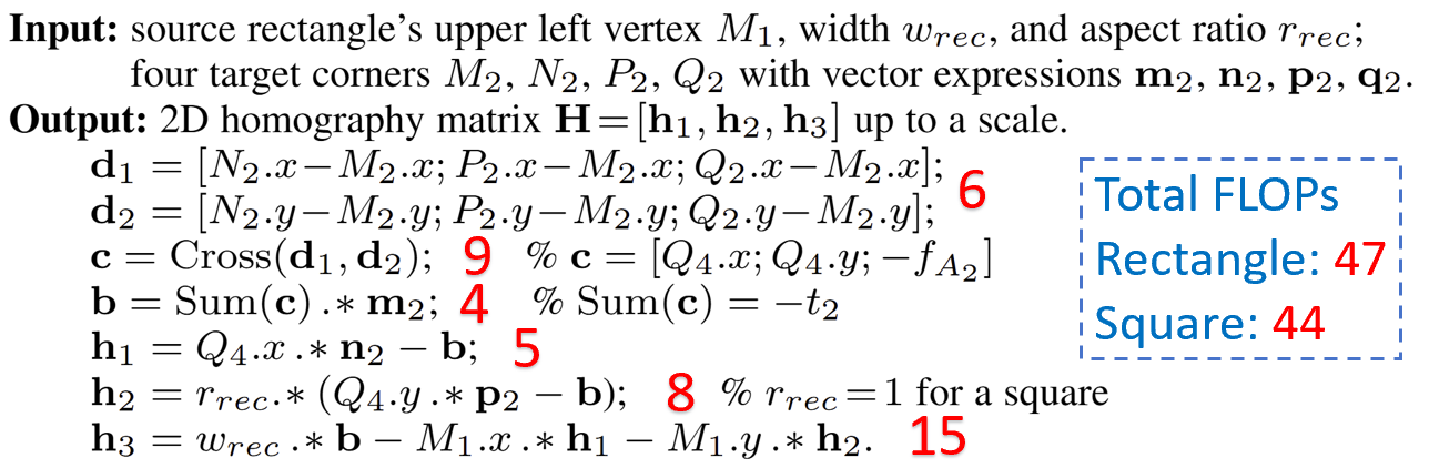
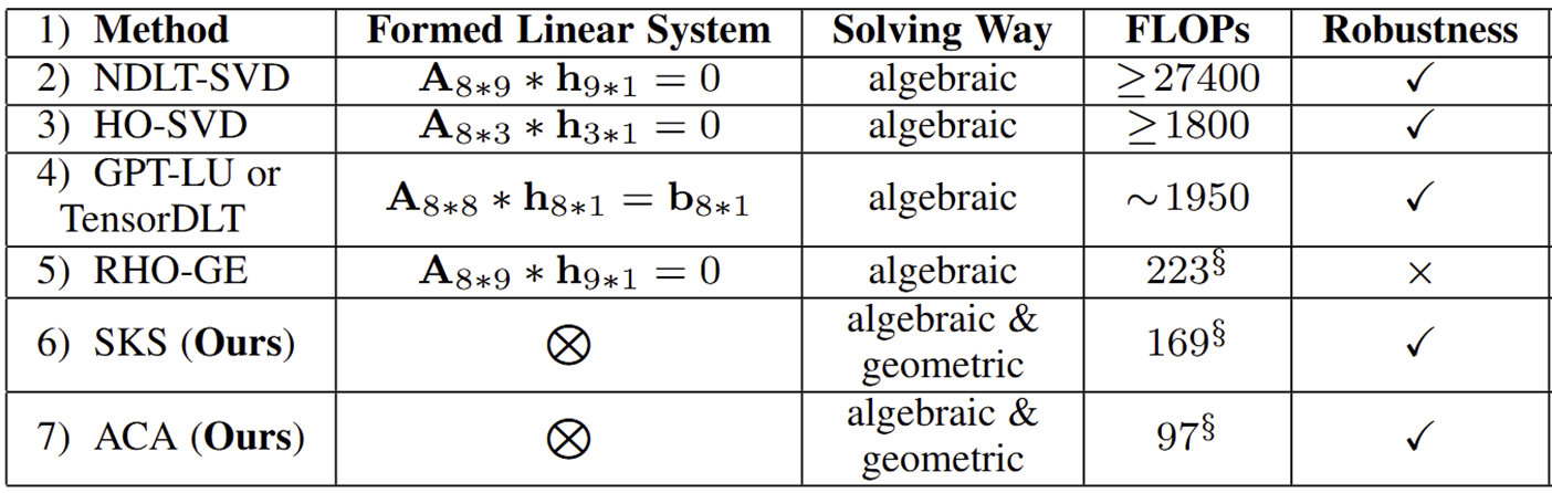
Fast and Interpretable 2D Homography Decomposition:
Similarity-Kernel-Similarity and Affine-Core-Affine Transformations

PAMI 2025


Shen Cai1*, Zhanhao Wu1,2, Lingxi Guo1,3, Jiachun Wang1,4, Siyu Zhang1,5, Junchi Yan6, Shuhan Shen7,8*,

1Visual and Geometric Perception Lab, Donghua University    2China Mobile (Hangzhou)    3ByteDance (Shanghai)    4Huawei (Shenzhen)   
5Microsoft (Redmond)    6School of Artificial Intelligence, Shanghai Jiao Tong University    7Institute of Automation, Chinese Academy of Sciences   
8School of Artificial Intelligence, University of Chinese Academy of Sciences

Core Idea


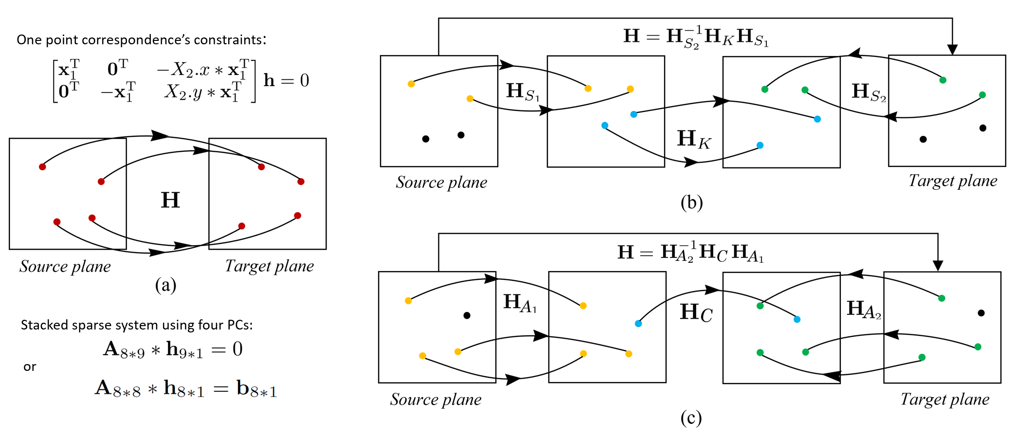
Previous 4-point homography methods indiscriminately utilize all four point correspondences to construct a sparse linear system, using the Direct Linear Transformation (DLT) strategy, as shown in (a). This system (with many 0s and 1s) is typically solved by standard matrix factorization techniques like LU decomposition based on Gaussian elimination. In contrast, our Similarity-Kernel-Similarity (SKS) and Affine-Core-Affine (ACA) decomposition tackle the homography geometrically, as depicted in (b) and (c). SKS uses two point correspondences (yellow and green) to estimate the two involved similarity transformations, while ACA employs three for affine transformations. The remaining points (blue) in each case address the residual projective distortion.


Similarity-Kernel-Similarity (SKS) Decomposition


The homography $\mathbf{H}$ between the source plane $\pi_1$ and the target plane $\pi_2$ is decomposed as \begin{equation} \mathbf{H} = \mathbf{H}_{S_2}^{-1}\mathbf{H}_K\mathbf{H}_{S_1}=\mathbf{H}_{S_2}^{-1}\mathbf{H}_{E}^{-1}\mathbf{H}^{'}_{S}\mathbf{H}_{E}\mathbf{H}_{S_1}=\mathbf{H}_{S_2}^{-1}\mathbf{H}_{E}^{-1}\mathbf{H}_{T_2}^{-1}\mathbf{H}_{G}\mathbf{H}_{T_1}\mathbf{H}_{E}\mathbf{H}_{S_1} \end{equation}

where $\mathbf{H}_{S_1}$ and $\mathbf{H}_{S_2}$ are similarity transformations normalizes the source and target planes, respectively; $\mathbf{H}_{K}$ with four degrees of freedom (DOF) induces the projective distortion between two normalized planes $\pi_3$ and $\pi_4$; $\mathbf{H}_{E}$ denotes an elementary transformation, mapping the points $[\mp1,0,1]^\top$ to the rectangular hyperbolic points $\{{I}^{'}\!,{J}^{'}\}$ ($=[\mp1,1,0]^\top$); $\mathbf{H}^{'}_{S}$ denotes the hyperbolic similarity transformation, which is further decomposed into two translations and $\mathbf{H}_{G}$ denoting hyperbolic rotation and scale.

The FLOPs for each step in SKS are given in the table below.


Affine-Core-Affine (ACA) Decomposition


The homography $\mathbf{H}$ between the source plane $\pi_1$ and the target plane $\pi_2$ is decomposed as \begin{equation} \mathbf{H} = \mathbf{H}_{A_2}^{-1}\mathbf{H}_C\mathbf{H}_{A_1}. \end{equation}

where $\mathbf{H}_{A_1}$ and $\mathbf{H}_{A_2}$ denote two affine transformations on the source and target planes, under which three general points are mapped to the canonical form $\{[0,0,1]^\top,[1,0,1]^\top,[0,1,1]^\top\}$; The core transformation $\mathbf{H}_C$ imposes the projective distortion between two affine normalization planes.

The FLOPs for each step in ACA are detailed in the table below, along with some additional details. Excluding last-element normalization, ACA achieves extreme efficiency, requiring only $\textcolor{red}{85}$ FLOPs per homography computation, free of division.


Polynomial Expression for Each Homography Element


Due to the avoidance of division, each element of a homography is expressed as a 7th to 9th degree polynomial in 16 input coordinates, as follows: \begin{equation} \mathbf{H} = \begin{bmatrix} h_{11}^{(8)} & h_{12}^{(8)} & h_{13}^{(9)} \\ h_{21}^{(8)} & h_{22}^{(8)} & h_{23}^{(9)} \\ h_{31}^{(7)} & h_{32}^{(7)} & h_{33}^{(8)} \end{bmatrix}. \end{equation}


Unified Solution to Affine Transformations


Leveraging ACA, an affine transformation $\mathbf{H}_{A}$ is decomposed as \begin{equation} \mathbf{H}_{A} \!=\! \mathbf{H}_{A_2}^{-1}\mathbf{H}_{A_1} \!=\! \begin{bmatrix} \overrightarrow{M_2N_2}.x & \overrightarrow{M_2P_2}.x & M_2.x \\ \overrightarrow{M_2N_2}.y & \overrightarrow{M_2P_2}.y & M_2.y \\ & & 1 \end{bmatrix} \begin{bmatrix} \overrightarrow{M_1P_1}.y & -\overrightarrow{M_1P_1}.x & \\ -\overrightarrow{M_1N_1}.y & \overrightarrow{M_1N_1}.x & \\ & & f_{A_1} \end{bmatrix} \! \begin{bmatrix} 1 & & -\!M_1.x \\ & 1 & -\!M_1.y \\ & & 1 \end{bmatrix}, \end{equation} where the kernel transformation $\mathbf{H}_{C}$ is an identity matrix and thus omitted; The FLOPs of computing $\mathbf{H}_{A}$ using our expression is only $\textcolor{red}{33}$ (7 for $\mathbf{H}_{A_1}$, 4 for $\mathbf{H}_{A_2}$, 14 for multiplication of the first two matrices, and 8 for residual multiplication).


Unified Solution to Versatile Image Primitives


SKS/ACA partially inherits from our previously proposed methods: EGED [MVA2013] and TPDH [IVC2017]. Therefore, SKS/ACA is equally applicable to various 2D primitives below, including two coplanar conics with real or imaginary intersections, four degenerate points, and one conic and one line.


Simplest Expression for Rectangle Pattern


When the four source points form a special shape, such as a rectangle or square, the linear system becomes sparser, leading to further simplifications in ACA. The following algorithm illustrates the computation process for a rectangular (or square) pattern, requiring $\textcolor{red}{47}$ and $\textcolor{red}{44}$ FLOPs, respectively.


$\textcolor{red}{\textbf{Note:}}$ When a square is used for camera calibration (focusing on intrinsic parameters) or QR code detection, the location of the planar coordinate system is often irrelevant. A simple setup assumes the upper-left vertex as the origin ($M_1.x=0$, $M_1.y=0$) and the square's side length as $w_{rec} = 1$. In this case, the computation of $\mathbf{h}_3$ is avoided (due to $\mathbf{h}_3=\mathbf{b}$), further simplifying the homography computation to $\textcolor{red}{\textbf{29}}$ FLOPs.


Experimental Results


1. Theoretical FLOPs

Before presenting the experimental results on runtime, we revisit FLOPs of previous methods and our approach, as shown in the table.


2. Runtime on CPU

In experiments on CPU, SKS and ACA offer significant advantages in speed due to our concise calculations. The fastest ACA (*) achieves approximately 70 million runs per second on the CPU.

Od: turns off all compiler optimizations
O1 & O2: a combination of optimizations including vectorization (SIMD)
(*) & (**): implementation with single-precision and double-precision floating-point numbers


3. Runtime on GPU

Considering that homography computation can be parallelized in a RANSAC framework, we conducted experiments on a GPU. It is observed that the total runtime for all algorithms, when computing no more than 10,000 homographies, increases slightly as the number of computations rises. This is because parallel computation of a small number of homographies does not trigger all CUDA cores. When one million homographies are required, the fastest ACA achieves approximately 4 billion runs per second on the GPU.


Conclusion


To the best of our knowledge, the proposed method demonstrates extreme efficiency and offers various distinct advantages, as elaborated above. In our view, $\textbf{SKS/ACA constitutes a comprehensive solution for plane-based geometric vision problems}$. Additionally, SKS/ACA shows potential for extension into projective geometry and computer graphics. Interested readers are encouraged to further explore its extensive possibilities.


  CASH Reward